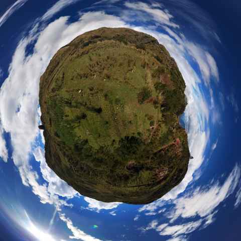
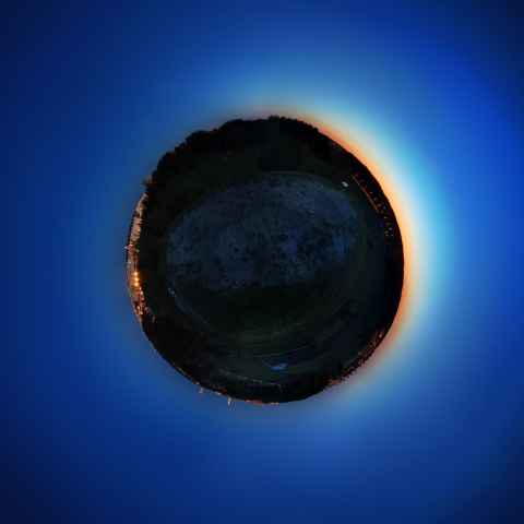
Planet Bigshot

While playing around with Stellarium[a], I noticed that if you looked straight down, the ground would roll up into a small "planet" in the center of the screen. When I made the Granholmstoppen Stellarium Landscapes, I decided I wanted to create preview images that looked like little planets. So, I got on with it, and added a bigshot.MakePlanet class to Bigshot.

​1. Theory

The "planet" projection is quite simple. You load an equirectangular map, and for each point in the output square, you determine its polar coordinates,  theta  (the angle) and  rho  (the distance from the center). Then we set  phi = f(rho)  and use the resulting  phi  to look up a pixel in the equirectangular map. The trick to getting a good output image, as I noticed, is to pick a good function to map distance from the center of the image to the angle  phi .

​2. The Mapping

If the mapping from  rho  to  phi  is linear, then the output image is dominated by the view straight down, and everything interesting on the horizon would be squashed into a thin ring outlining the planet. I wanted some way to stretch the image around the horizon, and so I settled on a piecewise curve. First, I normalized the distance from the center of the image to the nearest edge (half the width of the image) to the interval  [0, 1] . This placed the corners at  sqrt(2) . Second, we'll also normalize the range of  phi  to  [0, 1] , for simplicity's sake.

Then I could select a point at which the "stretch" would be at its maximum, and the amount of stretch. Let's call this point  P , with  P_(rho)  being the point where the stretch is the maximum, and  P_(phi)  is the output of the function at that point. This gives us a piecewise function with two intervals, let's call them  phi_(g)  for ground and  phi_(s)  for sky. We also decide where we want to place the zenith - should the planet be a disc that just about touches the edges of the square, or should it cover the image? If the former, we set  rho_(max) = 1 , if the latter  rho_(max) = sqrt(2) ~~ 1.42 .

Since the function must be continuous and map to  [0, 1] , we get the constraints:

Then, choosing an exponent for each -  c_(g)  and  c_(s) , respectively - the two functions become:

Stopping here and using  phi_(p)  worked out OK, but I still had the problem that I got an ugly "pinch" effect in the center of the image, as the  phi  values would climb so fast there. So I blended the output with a linear mapping from zero to  L_(max) :

Which is a simple linear blend on the interval  [0, L_(max)] . The result looks like this:

We can see that the output climbs sharply only to level off around 0.5, which is where we find the horizon, and the continues to climb all the way to  rho = rho_(max) = 1.42  (the corners) where  phi = 1  and we look straight up.

To see the amount of "stretch", it's helpful to plot the inverse of the derivative of φ with respect to ρ:

High values means that we sweep through the angles slowly (much stretch), while a low derivative means that we move quickly (little stretch). As we can see, the stretch reaches its minimum at 0.5, which is precisely at the horizon and my choice for  P_(rho) . The other parameters are  P_(phi) = 0.5 ,  L_(max) = 0.5 ,  c_(g) = 1/3 ,  c_(s) = 1.2  and  rho_(max) = 1.42 .

​3. Example Images

Tambomachay
Cusco, Peru

Bigshot, Tambomachay

Granholmstoppen
Stockholm, Sweden

Bigshot, Granholmstoppen

Lilla Slingan
Stockholm, Sweden

Bigshot, Lilla Slingan

Tawi Hassain
Dubai Desert Conservation Reserve, Dubai

Bigshot, Tawi Hassain